This is not like other Codechef questions but still very interesting.
How do we find lowest common ancestor in Binary Tree in O(n) time provided that you do not have any extra memory to store parent pointer at every node?
↧
Finding lowest common ancestor in Binary Tree
↧
Finding range overlap of maximum weight
You are given a list of size N, initialized with zeroes. You have to perform M queries on the list and output the maximum of final values of all the N elements in the list. For every query, you are given three integers a, b and k and you have to add value k to all the elements ranging from index a to b(both inclusive). Input Format First line will contain two integers N and M separated by a single space. Next M lines will contain three integers a, b and k separated by a single space. Numbers in list are numbered from 1to N. Output Format A single line containing maximum value in the final list. Constraints: 3 <= N <= 10^7, 1 <= M <= 2 * 10^5, 1 <= a <= b <= N, 0 <= k <= 10^9
Sample Input:
5 3
1 2 100
2 5 100
3 4 100
Sample Output:
200
What can be the most efficient approach to solve this problem?
↧
↧
Submission result not coming
Hi,
Image may be NSFW.
Clik here to view.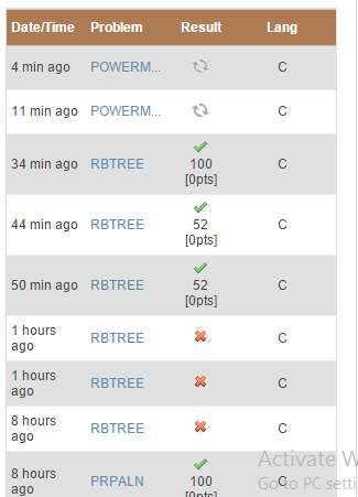
I am not aware what's the problem is, My submissions are not getting any results from last 10-12 mins.
EDIT: 34 MINS
↧
SPOJ AIBOHP
http://www.spoj.com/problems/AIBOHP/
Googled this question. Many people have the same solution. But i am getting runtime error only.
Can anyone help??
↧
NOV14- SPELL problem
I'm not clear with how the input is given and also the output.
The input says you will be given D lines each containing a word. After that there will be a line.
So in the output do we have to correct just that line.(which is after D lines in input)
Or we have to correct every word given in D lines in input.
It also says "Output the corrected text in the same format as it is given to you in the input." Does that mean our ouput will also contain D lines containing corrected word(if erroneous).
↧
↧
PRPALN- Subtask-1 35 points or 65 ?
The constraints as given in the problem statement state subtask -1 score 65 points. My submission scores me 35 points for subtask -1 on AC. Is that a miss-print in the constraint description?
Image may be NSFW.
Clik here to view.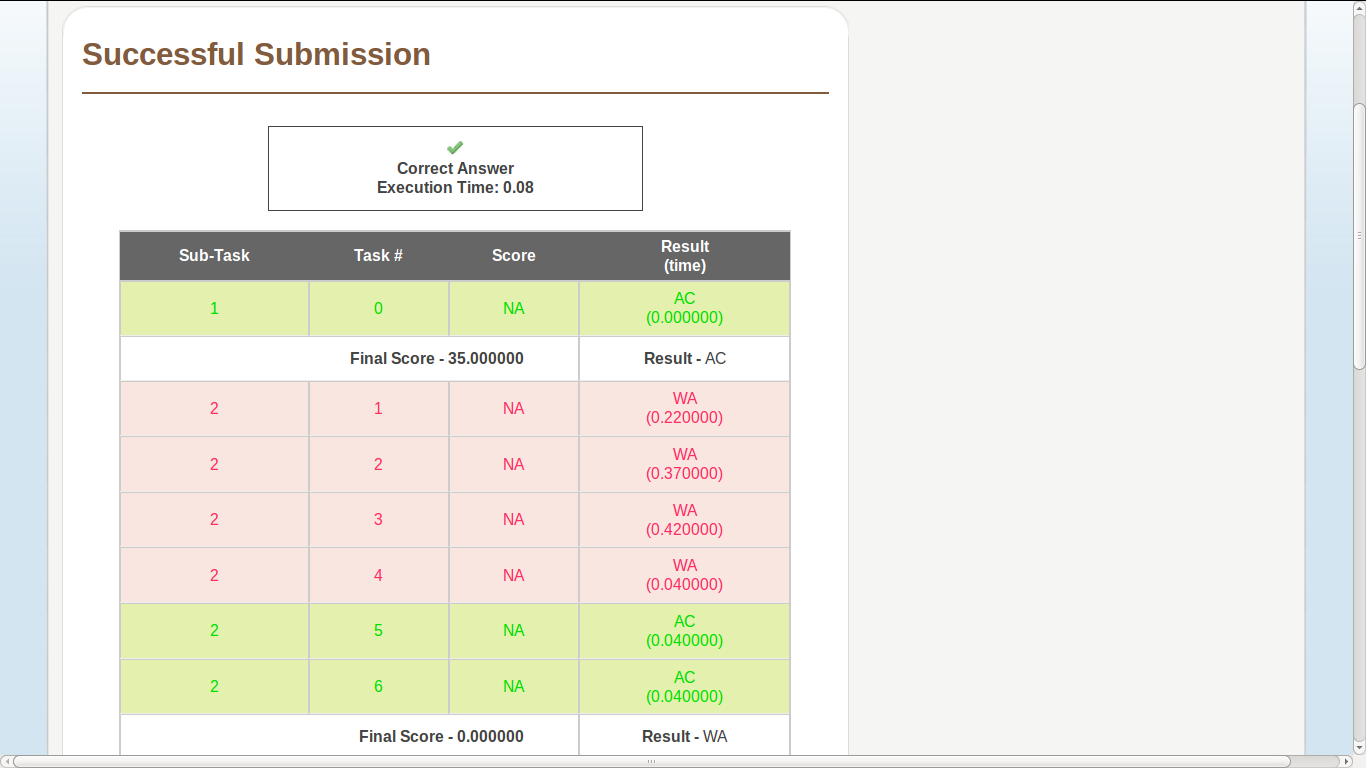
↧
Time Limit Exceeded
Hey! I was asked this question in my C-Programming assignment in college. I tried submitting a solution but got TLE. Could anybody please tell me how I could optimize it? Just give me a hint or what I have to use. I want to do it on my own. Thanks! Here goes the question :
We all know what Fibonacci numbers are (The sequence of numbers such that every number in the sequence is the sum of the previous two numbers in the sequence, with the first two numbers 0 and 1)
f(n) = f(n − 1) + f(n − 2) f(1) = 0 f(2) = 1
Now lets define a new kind of Fibonacci numbers, the iFibo Numbers.
The iFibo numbers are defined as the sequence of numbers, such that every number in the sequence is the sum of A times the previous number, B times the number before the previous number, and C times the number before the number before the previous number in the sequence, with the first two iFibo numbers equal to D, E and F.
f(n) = A * f(n − 1) + B * f(n − 2) + C * f(n − 3)
f(1) = D f(2) = E f(3) = F
Now, your task is simple. Given N, A, B, C, D, E, F you need to tell the Nth iFibo number (mod 10000007).
Input
The first line contains T. Next T lines contain 7 space separated integers N A B C D E F.
Output
For each testcase, output in a single line, the Nth iFibo number, mod 10000007.
Constraints
0 <= A, B, C, D, E, F < 10000007
For 80% score
0 <= T <= 50
1 <= N <= 100000
For 100% score
0 <=T <= 100000
1 <= N <= 10^12
SampleInput
3
5 1 1 0 1 1 2
4 1 1 1 1 1 1
10 2 0 2 1 2 3
Sample output
5
3
1424
↧
No score in "The Spelling Problem" of november long
In Nov long partial problem my solution is getting accepted but not producing any score not even 0. It is running fine on my computer. In fact this is happening when I am trying to include the case of character skipped(read link text) without which it is producing some score.
Image may be NSFW.
Clik here to view.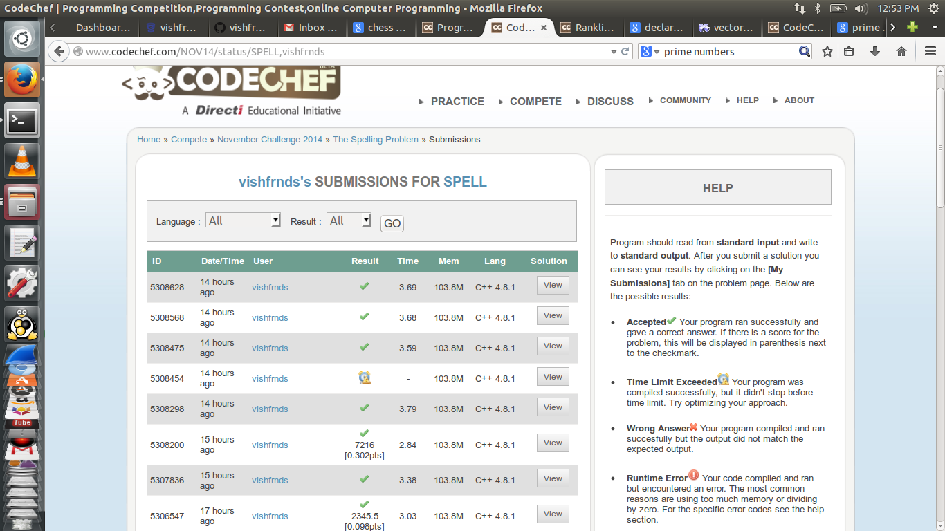
↧
game theory
Given an array of positive numbers. There are two players A and B. In his/her turn a player can pick either one or two elements from the front end of the array and these elements are then removed from the array. Players play alternately In the end values the players are holding are summed up. The player with larger sum value wins. If both play optimally, find who wins e.g. 5 {1 1 0 0 1} A wins , 6 {1 5 6 3 2 9} B wins 4 {1 1 1 1} Game draws
↧
↧
string length
how to input a string of length n where 1<=n<=100000 ?
↧
DISCHAR question
Are the characters ASCII characters or UNICODE?
↧
Does CodeChef have any Code Of Conduct?
I am new to CodeChef. I am not sure what can be considered as an improper conduct on this website. I do not want to be penalized for doing something unknowingly which is not the accepted behavior. Is there any such Code of Conduct?
↧
Timings of ICPC onsite regional contests
What are the exact timings for the ACM ICPC onsite regional contests, both the practice and the main contest for all the three sites. Please share an official source if possible.
↧
↧
QSTRING-Editorial
PROBLEM LINK:
Author:Minako Kojima
Tester:Jingbo Shang
Editorialist:Ajay K. Verma
DIFFICULTY:
Medium
PREREQUISITES:
Suffix Array, LCP Array, Persistent Segment Tree
PROBLEM:
Given a string S, support the following queries:
1) Given integers k1 and k2, compute the k1-th lexicographic smallest substring S1 among all unique substrings of S. The substring S1 may occur several times in S, find its k2-th occurrence.
2) Given a substring S[l..r], find its rank k1 among the unique substrings of S, Also this substring may occur several times in the string, find how many of these substrings start before l.
EXPLANATION:
First let us ignore the k2, and instead consider a simpler problem, which supports the following two queries:
1) Given k1, find the k1-th lexicographic smallest substring S1 among all unique substrings of S.
2) Given a substring S[l..r], find its rank k1 among the unique substrings of S.
The two queries can be answered easily using the suffix array and lcp array of the string S. In order to see the construction algorithm for suffix and lcp array consider looking at this.
Briefly, suffix array of an string S[1..N], consists of of an array SA[1..N], where SA[i] is the index x such that S[x..N] is the i-th lexicographically smallest suffix of string S. Usually, we also create the inverse array of SA, known as POS[1..N]. The element POS[i] gives the rank of suffix S[i..N] among all suffixes of S.
the lcp array lcp[1..N] is used to compute the longest common prefix of suffixes of S. The value lcp[i] represents the length of the longest common prefix of the suffix S[SA[i]..N] and S[SA[i - 1]..N] for i > 1. A combination of lcp array and range minimum data structure can be used to compute the length of the common prefix of arbitrary suffixes of S in O(1) time as shown here.
Unique Substrings:
Suffix array can be used to compute the number of unique substrings of S. We count these substrings in lexicographic order. Since the array SA[] consist of the string indices in lexicographic order of suffixes, hence, in the lexicographic enumeration of unique substrings of S, the substrings starting at SA[i] will be counted before counting the substrings starting at SA[j] for i < j.
Suppose we are considering the substrings starting at index SA[i]. There are (N + 1 - SA[i]) such substrings, however, many of these substrings have already been counted. More specifically, if the length of the longest common prefix of suffix starting at index SA[i] and the suffix starting at SA[i - 1] is x, then x of these (N + 1 - SA[i]) substrings have already been counted. So the number of additional substrings will be (N + 1 - SA[i] - x) = (N + 1 - SA[i] - lcp[i]).
Adding these values together will give us the number of unique substrings of S. Now, let us create an array substr[1..N], such that substr[i] gives the number of unique substrings that have been counted after considering the suffixes starting at SA[1], SA[2], ..., SA[i].
substr[1] = N + 1 - SA[1],
substr[i] = substr[i - 1] + N + 1 - SA[i] - lcp[i]
Using the array substr[], we can compute the k1-th lexicographic smallest substring easily. Basically, we perform a binary search for k1 in the array substr[]. Let us say substr[i - 1] < k1 <= substr[i], this means the k1-th smallest substring must start at SA[i]. More specifically, the substring will be S[l..r], where,
l = SA[i]
r = SA[i] + lcp[i] + k1 - substr[i - 1]
On the other hand, if we want to compute the rank of substring S[l..r], we need to find out when this substring was considered in the enumeration of unique substrings. Suppose this string was counted for the first time when we were considering the substrings starting at SA[x], that means x is the smallest index such that the suffix starting at SA[x] contains S[l..r] as a prefix, i.e., the the length of the longest common prefix of the suffix starting at l and SA[x] is >= (r - l + 1).
Since the suffix starting at index l contains the substring S[l..r] as a prefix, x must not exceed POS[l]. Moreover, for all x <= y <= POS[l], the length of the longest common prefix between the suffix starting at SA[y] and the suffix starting at l will be >= (r - l + 1). Hence, x can be found using a binary search.
Once we have found x, the rank k1 can be found easily. In fact the rank k1 will be
k1 = substr[x - 1] + (r - l + 1) - lcp[x]
This means using the suffix and lcp array, we can handle the simplified queries in O (lg N) time. Next, we discuss how to handle the queries which also consider the ranking of same substring based on their starting points.
Ranking of Substrings based on Starting Index:
Suppose that we are handling the first query, where k1 and k2 are given and we want to compute the substring S[l..r]. Using the algorithm described in previous section, we can easily find one occurrence of this substring, which is at
l = SA[i]
r = SA[i] + lcp[i] + k1 - substr[i - 1]
where i is the smallest index such that substr[i] >= k1.
Note that the substring S[l..r], will occur at position x, iff the length of the longest common prefix of the suffix starting at x and the suffix starting at l is >= (r - l + 1). We need to find all such x's. It can be seen that the set of these x's will be of the form
{SA[low], SA[low + 1], ..., SA[i], ..., SA[high - 1], SA[high]}
The value of low and high can be computed using binary search and the lcp computation. Once, we have the set of all possible x's, we need to find the k2-th smallest value among these. We will discuss how to do this efficiently a bit later. First let us discuss how to handle the second type of query.
For the second query, we are given the substring S[l..r]. Using the method described in previous section, we can compute its rank k1 in O (lg N) time. This substring will occur many times in the string, and the starting indices of these occurrence will form the set
{SA[low], SA[low + 1], ..., SA[POS[l]], ..., SA[high - 1], SA[high]}.
Here also the value of low and high can be computed using a binary search, and we want to compute the rank of SA[POS[l]] in this set, which will be the value of k2.
Persistent Segment Tree:
In the above section we have seen that the problem of handling the two kind of queries finally reduces to design a data structure that supports rank and select queries on the subarray. More specifically,
Given an array SA[1..N], design a data structure structure that supports the following queries:
1) Given l, r, and k find the k-th smallest element in the subarray SA[l..r]
2) Given l, r, and x, find the rank of x in the subarray SA[l..r].
The data structure that handles these queries efficiently is known as Persistent Segment Tree, which can handle the two queries in O (lg N) time. The details of this data structure can be seen at here and here (in Russian, I guess).
Hence, we can handle the two kind of queries in O (lg N) time.
Time Complexity:
Preprocessing time: O (N lg N)
Query time: O (lg N)
Weak Test Cases:
Unfortunately, the test cases for this problem were weak (or the time limit was too relaxed), that allowed O (QN) solutions to run in time. Some contestants informed the admins about this during the contest, however, those mails slipped through the cracks, and the setter never became aware of this issue during the contest. The setter has now added the strong test cases, which are available in practice section. However, at this point it does not seem possible to rejudge all accepted solutions.
AUTHOR'S AND TESTER'S SOLUTIONS:
Author's solution will be put up soon.
Tester's solution will be put up soon.
↧
BTREE-Editorial
PROBLEM LINK:
Author:Tom Chen
Tester:Jingbo Shang
Editorialist:Ajay K. Verma
DIFFICULTY:
Hard
PREREQUISITES:
Tree Partition, Lowest Common Ancestor, Persistent Segment Tree
PROBLEM:
We are given a tree with N nodes. We need to process the queries of the following type: for a given set S = {v1, v2, ...vk} of k nodes, and a set of k integers {d1, d2, ..., dk}, find the number of nodes in the tree which are within di distance from the node vi, for some i.
EXPLANATION:
We will first solve an easier version of the problem where all queries have k = 1, and then use it to solve the case for general k.
Queries with k = 1:
In this case the queries will be of the form: given a node v and an integer d, find the number of nodes which are within d distance from v. As a notation we will call d as range of node v.
Balanced Tree:
Let us further simplify the problem, and assume that the given tree is a rooted balanced tree, i.e., for each node the subtrees rooted at its child nodes are similar in size.
We preprocess the tree, and compute the depth (distance from root node) of all nodes in the tree. We also associate a special data structure (which we name as "depth profile" of the subtree) at each node, the pointer of this structure is stored at all nodes in the subtree rooted at this node.
Suppose, we want to create the depth profile of the subtree rooted at node v. Let us say that node v has m children namely u1, u2, ..., um. The depth profile of the subtree contains (1 + m) vectors. The first vector A[] stores the global information of the tree, while the remaining m vectors B[1..m] store the information about the subtree rooted at children nodes. More specifically
A[i] = number of nodes in the subtree rooted at v, which are within distance i from v,
B[i][j] = number of nodes in the subtree rooted at ui, which are within distance j from v.
depth_profile(v) = {A, B[1], B[2], ..., B[m]}
Each node in the subtree rooted at v, stores the following information:
1) pointer to depth_profile(v),
2) distance of this node from v,
3) the index of the child node ui, whose subtree this node belongs too, for the root node v, this index is 0.
Since the tree is balanced, each node will store the information about O (lg N) depth profiles, corresponding to the nodes which are in the path from root to this node.
Now, let us see how to use this information to answer the queries. Suppose for a given node w, we want to find the number of nodes within distance d from it. We look at all the depth profiles whose pointer is stored at node w.
Let us say we are looking at the depth profile of node v, which is an ancestor of w and is at a distance r from w, moreover w lies on the subtree of i-th child ui of v. Note that, all the nodes in the subtrees rooted at {u1, u2, ..., um} / {ui}, whose distance from v is smaller than (d - r), will be with d distance from w. The number of such nodes will be (A[d - r] - B[i][d - r]). So now we know the number of nodes within distance d from w, which are in the subtree rooted at v, but not in the subtree rooted at ui. If we consider the depth profile of all nodes in the path from root to w, and add the computed value, we will get the number of nodes within distance d from w.
The time taken to answer this query is O (number of depth profiles we looked at). Since the tree is balances, this will be O (lg N).
Lopsided Tree:
In case of a lopsided tree, the height of the tree could be O (N), and hence the query time also could be as large.
However, we can manipulate the root of the tree, so that we only need to store the pointer of O (lg N) depth profiles at a node. We pick the root node v in such a way that t(v) = max (size(u1), size(u2), ..., size(um)) is minimum, which will be the most balanced partition at this level. Also, for such v, t(v) <= m/2, where m is the number of nodes in the subtree rooted at v. Now for the depth profile of the subtree rooted at node ui, we can again manipulate the root, i.e., the root of this subtree does not need to be ui, but we will pick the one, which has the most balanced children subtrees. Since the depth profile of v is completely independent than the depth profile of ui, picking a different root for the subtree rooted at ui will not change anything.
This means that we can modify our data structure in a way that the queries for lopsided tree can also be answered in O (lg N) time.
General Queries (k >= 1):
If the given subset has k > 1 nodes, then we cannot just handle each of the k nodes independently, and add the values together, as some nodes of the tree might be counted several times.
For this reason, we partition the tree into k subtrees, each "centered" at one of the k nodes in the give subset. The partition will have the property that if a node lies in the partition centered at vi, and is in the range of one of the nodes of the subset (say vj), then it must also be in the range of vi. The property is important because it says that we can handle the partitions independently, and for each partition we only need to find the nodes which are reachable in the specified distance from the center of the partition.
Tree Partition:
First we create an auxiliary tree with O (k) nodes. This tree contains all the nodes in the given subset S as well as lowest common ancestors of some of the nodes of the subset. In the lack of a picture, lets try to understand this with the help of an example.
Suppose the given tree (rooted at 1, for simplicity) has the following edges:
(1, 2), (1, 3)
(2, 4), (2, 5), (2, 6),
(3, 7), (3, 8),
(6, 9), (6, 10)
If the chosen subset S is {1, 4, 6, 7}, then the auxiliary tree will have the nodes {1, 2, 4, 6, 7}, and the following edges:
(1, 2), (1, 7),
(2, 4), (2, 6).
Note that (1, 7) is an edge which was not present in the original tree. In the general case the edges in the auxiliary tree correspond to the "monotonic path" (a path between a node and its ancestor) in the original tree.
The auxiliary tree can be created easily using a stack. We already have the nodes of the tree in depth first traversal order, as well as a data structure which can answer the lowest common ancestor queries efficiently (you can refer to this editorial to know more about this data structure). In order to compute the additional nodes of the auxiliary tree, we need to traverse the nodes of the subset in the tree depth first traversal order, and add the lowest common ancestor of any two consecutive nodes in the subset.
In the above example the nodes in depth traversal order are (1, 4, 6, 7), we need to add lca(1, 4) = 1, lca(4, 6) = 2, lca(6, 7) = 1, in the auxiliary tree. Hence, the auxiliary tree will have {1, 2, 4, 6, 7} as nodes.
In order to create the edges of the auxiliary tree, we traverse its nodes in the depth first traversal order (of the the original tree), while maintaining a stack of visited nodes. Since we are visiting nodes in the depth first traversal order, if an already visited node u is not an ancestor of current node v, it will never be ancestor of any node visited in future, so we can remove it from the stack. On the other hand, if u is an ancestor of v, then we create an edge (u, v). The following snippet shows the pseudocode of the same.
void CreateEdges(vector<int> &nodes) {
    stack st;
    for (int v : nodes) {
        while (!st.empty()) {
            int u = st.back();
            if (u is an ancestor of v)
            {
                addEdge(u, v);
                break;
            }
            st.pop();
        }
        st.push(v);
    }
}
In our example, the process goes as follows:
visited nodes = {}
stack = {}
visited nodes = {1, 2}
stack = {1, 2}
edge added = {(1, 2)}
visited nodes = {1, 2, 4}
stack = {1, 2, 4}
edge added = {(1, 2), (2, 4)}
visited nodes = {1, 2, 4, 6}
stack = {1, 2, 6}
edge added = {(1, 2), (2, 4), (2, 6)}
visited nodes = {1, 2, 4, 6, 7}
stack = {1, 7}
edge added = {(1, 2), (2, 4), (2, 6), (1, 7)}
Now, we have the auxiliary tree, we are ready to partition the tree. We label all the nodes in the auxiliary tree with one of the nodes in the given subset S, such that if label of node w is v, that means (range (v) - dist(v, w)) is largest among all nodes v in S. This implies that if w is within the range of any node in the S, then it must also be in the range of v.
Such a labeling can be obtained easily by running Dijkstra's algorithm on the auxiliary tree, as shown in the following snippet.
void Label() {
    max_heap H;
    for (int v : S) {
        H.insert(make_pair(range[v], v));
    }

    while (!H.empty()) {
        (d, u) = H.front();
        H.pop();

        for (v : neighbors(u) in the auxiliary tree) {
            r = dist(u, v);
            if (range[v] >= (d - r)) continue;

            range[v] = d - r;
            label[v] = u;
            H.insert(make_pair(d - r, u));
        }
    }
}
Now we know the range and label of all nodes in the auxiliary tree. However, the edges of this tree correspond to monotonic paths in the original tree. Hence, if the two end-points of an edge have different label, we need to find the exact partition of the edge. For example, if we have an auxiliary edge between nodes u and v (u is an ancestor of v), and the two nodes have labels x and y, then there will a node z in the path from u to v, such that all nodes in the path (u --> z) / {z} will have label x, while all nodes in the path (z --> v) will have label y.
Finding z is quite easy:
range[u] - dist(u, z) < range[v] - dist(v, z)
range[u] - range[v] < dist(u, z) - dist(v, z)
range[u] - range[v] < depth(z) - depth(u) - (depth(v) - depth(z))
range[u] - range[v] +depth(u) + depth(v) < 2 * depth(z)
(range[u] - range[v] +depth(u) + depth(v) + 1) / 2 = depth(z)
This uniquely identifies z.
In other words, all the nodes in the subtree rooted at u will come in the partition centered at x, except the ones which are in the subtree rooted at z, which will come in the partition centered at y.
If u is the root of the auxiliary tree, then not only the nodes in the subtree rooted at u, will be in x's partition, but also the ones which are outside the subtree.
Handling the Query:
After the partition, we go through the nodes of the auxiliary tree. For each node u, we already know its label and range. Next, we compute the number of nodes of the original tree, which are within range of this node, and belong to the same partition as this node. We show the steps involved in this process below.
1) Consider the auxiliary edge (parent[u], u), partition this edge into two sub edges (parent[u], z) and (z, u) as explained in the previous section. Compute the number of nodes in the subtree rooted at z, which are within range[u] distance from u, and add them to the answer. If node u has no parent, then consider z to be the root of the original tree.
2) Consider each auxiliary edge (u, v), partition the edge into (u, z) and (z, v). Compute all nodes in the subtree rooted at z, which are within range[u] distance from u, and subtract this from the answer.
Since, we are subtracting the nodes, which belong to different partition, a node is counted only for one partition. Hence, this will give the right answer.
However, in the above computation, we needed to handle several queries of the form: Number of nodes in the subtree rooted at z, which are within d distance from a node u. Next, we show how to handle these queries.
There could be three possible cases:
1) neither u is ancestor of z, nor z is ancestor of u: In this case the number of nodes will the same as the number of nodes which are at a distance (d - dist(u, z)) from z.
2) u is ancestor of z: In this case also the number of nodes will be the same as the number of nodes which are at a distance (d - dist(u, z)) from z.
3) z is ancestor of u: In this case we first compute the number of nodes at distance d from u (not necessarily in the subtree rooted at z). This can be computed as explained in the section handling the case of (k = 1). Since not all these nodes will be in the subtree rooted at z, we need to subtract the ones which are outside the subtree. Number of these nodes will be (number of nodes at distance (d - dist(u, z)) from z - number of nodes in the subtree rooted at z, which are at distance (d - dist(u, z)) from z).
This means, we only need to handle the queries of the form: find the number of nodes in the subtree rooted at z, which are at a distance d1 from z, i.e., the nodes in the subtree whose depth does not exceed (depth(z) + d1).
If we create a list of all nodes in the depth first order traversal, the nodes in a subtree correspond to an interval in the list. Hence, the above query translates to finding the number of element in a subarray, which are smaller than a given value. This is a classical data structure problem, which can be solved using Persistent Segment Tree in O (lg N) time.
Hence, the queries can be answered in O (k lg N) time.
Time Complexity:
Preprocessing time: O (N lg N)
Query time: O (k lg N)
AUTHOR'S AND TESTER'S SOLUTIONS:
Author's solution will be put up soon.
Tester's solution will be put up soon.
↧
PRPOTION-Editorial
PROBLEM LINK:
Author:Praveen Dhinwa
Tester:Jingbo Shang
Editorialist:Ajay K. Verma
DIFFICULTY:
Easy
PREREQUISITES:
ad-hoc, basic math
PROBLEM:
Given three arrays of positive integers, minimize the maximum element among the three arrays by performing the operation at most M times, where in an operation, all elements of a single array can be halved.
EXPLANATION:
A single operation halves all elements of the array. Hence, the index of the maximum element in the array will remain the same after the operation. This is because of the following observation:
x <= y ==> floor(x/2) <= floor(y/2)
Since, we are only interested in the maximum value after the operations, we do not need to consider all elements of the array, but only its maximum element. Hence, the problem reduces to the following: Given three integers (which are actually the maximum values of the three arrays), apply the operation at most M times such that the maximum of the three integers is minimum; a single operation halves one of the three values.
Order independence and Greedy Approach:
Note that the order in which we apply the operations does not matter as long as the number of operations applied on the three integers remain the same (respectively). In other words, if the initial values of the three integers is (x, y, z) and the number of operations applied on them are (a, b, c), then their final values will be (x/2a, y/2b, z/2c), no matter in which order we apply these operations.
If the value of the three integers is x >= y >= z, and we have some operations left, then at least one of the remaining operations has to be applied on x, otherwise the maximum of the three integers will not change. Since the order in which operations are applied does not matter, we should apply the very first operation on x. This gives us a greedy approach: In each step we should apply the operation on the largest of the three values. The following snippet shows the pseduocode for the greedy approach.
int min_val(int *R, int *G, int *B, int M) {
    int x = max(R);
    int y = max(G);
    int z = max(B);

    int arr[] = {x, y, z};
    for (int i = 1 to M) {
        sort(arr);

        // Apply the operation on the largest element
        arr[2] /= 2;
    }
    sort(arr);
    return arr[2];
}
Time Complexity:
O (N + M)
Remark about the Original Problem:
In the original version of the problem, a single operation not only halves the elements of a single array, but also increments the elements of other arrays by one.
It can be seen that here the order of operations is relevant, and different order may lead to different results. e.g.,
(5, 3, 1) --> (2, 4, 2) --> (3, 2, 3) --> (4, 3, 1)
(5, 3, 1) --> (6, 1, 2) --> (7, 2, 1) --> (3, 3, 2)
Hence, a greedy approach in this case will not lead to the optimal approach. For the initial set of numbers (7, 8, 4) and number of allowed operations <= 3, the greedy approach will produce 6 as answer.
(7, 8, 4) --> (8, 4, 5) --> (4, 5, 6) --> (5, 6, 3)
while the optimal solution is 5
(7, 8, 4) --> (3, 9, 5) --> (4, 4, 6) --> (5, 5, 3)
A dynamic programming based solution can be used in this case to solve the problem. However, the constraints in the problem were too high for that to run in time.
AUTHOR'S AND TESTER'S SOLUTIONS:
Author's solution will be put up soon.
Tester's solution will be put up soon.
↧
CHEFPNT-Editorial
PROBLEM LINK:
Author:Dmytro Berezin
Tester:Jingbo Shang
Editorialist:Ajay K. Verma
DIFFICULTY:
Challenge
PREREQUISITES:
Ad-hoc, Randomized Algorithm
PROBLEM:
We are given an N x M rectangle, where some of the cells are already colored. The goal is to color the remaining cells in minimum number of steps, where in a single step a maximal set of contiguous uncolored cells, aligned horizontally or vertically, can be colored.
EXPLANATION:
This is a challenge problem and there is no exact solution. A greedy algorithm could be to scan the cells in a row major order, and whenever an uncolored cell is encountered, either color a maximal row starting at this cell, or color a maximal column starting at this cell, whichever colors most number of cells.
void greedy() {
    for (int i = 1 to N) {
        for (int j = 1 to M) {
            if (a[i][j] is colored) continue;

            int x = 0;
            for (int k = j to M) {
                if (a[i][k] is colored) break;
                ++x;
            }

            int y = 0;
            for (int k = i to N) {
                if (a[k][j] is colored) break;
                ++y;
            }

            if (x > y) {
                for (int k = j to (j + x))
                    color(a[i][k]);
            } else {
                for (int k = i to (i + y))
                    color(a[k][j]);
            }
        }
    }
}
Of course there is no reason to traverse the cells in row major order, one could also traverse them in a column major order, or in decreasing row/column major order. Apply the greedy approach for each of them and pick the one which uses minimum number of steps.
We could go even further: After each coloring, we can pick one of the four traversal orders randomly, and then traverse the rectangle cells in that order to find the first uncolored cell. We can run this randomized version of greedy approach as long as time permits, and then pick the one which gives the best result.
In order to increase the number of random trials, we may want to increase the speed of our greedy approach. There are three main steps in the greedy approach:
1) find the first uncolored cell: could take O (NM) time, however, if we store the pointer from the previous iteration, it will take O (1) amortized time.
2) find the length of the maximal uncolored row/column starting at this cell: could take O (N + M) time,
3) color the row/column: could take O (N + M) time.
If we use (N + M) segment trees, one for each row and one for each column. The complexity of some of the steps can be reduced. The first step can be reduced to O ((N + M) lg (N + M)), the second step can be reduced to O (lg (N + M)), while the complexity of the third step will increase to O ((N + M) lg (N + M)).
One could also try representing the rows and columns of rectangle using bit masks, and use bit twiddling tricks to perform the three steps, which will also reduce the runtime of a single trial.
I did not manage to look at the top solutions very carefully, and it would be great if people could come forward and explain their approaches.
AUTHOR'S AND TESTER'S SOLUTIONS:
Author's solution will be put up soon.
Tester's solution will be put up soon.
↧
↧
PRLADDU-Editorial
PROBLEM LINK:
Author:Praveen Dhinwa
Tester:Jingbo Shang
Editorialist:Ajay K. Verma
DIFFICULTY:
Easy
PREREQUISITES:
ad-hoc, basic math
PROBLEM:
Given equal number of red (villager) and blue (dinosaur) points on a straight line (multiple points can share the same location), join each red point with a unique blue point by a line such that the sum of lengths of all lines is minimum.
EXPLANATION:
We first compute the lower bound on the total length on lines, and then show that the lower bound is in fact achievable.
Lower Bound on the Total Length:
Suppose we pick a point p on the line which does not coincide with any of the red or blue points, now let us find out the minimum number of lines that will pass through this point in any arrangement.
Let us say that there are r red points and b blue points on the left of point p, then there can be two cases:
1) r >= b. This means we have (r - b) extra red points to the left of p, these points can only be connected to the blue points on the right of p. Hence, there will be at least (r - b) lines that will cross the point p, and will join the blue points on the right of p.
2) r < b. In this case at least (b - r) lines will cross the point p, and will join red points on the right of p.
In other words at least |r - b| lines will cross the point p, which is the absolute difference between the red and blue points on the left of p. Now, we can consider all intervals between two consecutive point locations, and find the minimum number of lines containing these intervals.
In the problem we are given an array D[], such that if D[i] is non-negative that means there are D[i] red points at (i, 0), otherwise there are -D[i] blue points at (i, 0).
Now consider the interval between the points (i, 0) and (i + 1, 0). Based on the above observation, it can be seen that there will at least |D[1] + D[2] + ... + D[i]| lines crossing this interval (Note that D[i] values are signed, hence their sum computes the difference between red and blue points).
Minimum length of lines = \Sum (minimum number of lines crossing the interval [(i, 0), (i + 1, 0)]), where the sum goes over i from 1 to (N - 1), N being the size of array D.
The following pseudocode can compute this bound in linear time.
int64_t bound(int *D, int N) {
    int64_t ans = 0;
    int64_t curr = 0;

    for (int i from 1 to N) {
        curr += D[i];
        ans += abs(curr);
    }
    return ans;
}
Lower Bound is Achievable:
Now we show that the lower bound computed in the above section is in fact achievable.
We use the following strategy to create lines: Start from the leftmost location (1, 0) and create |D[1]| active lines with source either red (if D[i] >= 0), or blue (if D[i] < 0), we extend these active lines to the right. Each time we encounter a location containing red or blue points, we either start more active lines or stop some of the active lines, using the following rules.
1) If the active lines have red (blue) sources, and the encountered points are also red (blue), then we start more active lines with source red (blue).
2) If the active lines have red (blue) sources, and we encountered blue (red) points, we will close as many active lines as possible by joining them to the encountered blue (red) points (hence, all closed lines will join a red and a blue point). If the number of encountered points is less than the active lines, we will still have active lines with red (blue) source, which will go further right. On the other hand, if the number of blue (red) points is higher than the number of active lines, then all active lines will be closed, and we might need to start new active lines with blue (red) sources, if some of the blue (red) points are unmatched.
It is easy to see that at any point the number of active lines is the absolute difference between the red and blue points encountered, which was in fact the minimum number of lines crossing a point. This means the lower bound is in fact achievable.
Time Complexity:
O (N)
AUTHOR'S AND TESTER'S SOLUTIONS:
Author's solution will be put up soon.
Tester's solution will be put up soon.
↧
FATCHEF-Editorial
PROBLEM LINK:
Author:Ishani Parekh
Tester:Jingbo Shang
Editorialist:Ajay K. Verma
DIFFICULTY:
Easy
PREREQUISITES:
ad-hoc, basic math
PROBLEM:
We are given a line of length N, where M lattice points (points with integer co-ordinates) have pre-defined color. Chef makes a walk along the line starting from any point and finishing at any point such that all points on the line are visited at least once. He can switch his traversal direction at any of the lattice points. After the traversal a point p in the line has the same color as that of the point with pre-defined color which was visited just before the last visit to p. The task is to find the number of coloring arrangements that can be achieved by different traversals.
EXPLANATION:
If a point has a pre-defined color x, then its final color will be x, no matter which traversal is chosen. If a point does not have a pre-defined color, and the first point of the left of it with pre-defined color has color x, and the first point on the right with pre-define color has color y (note that in some cases x or y may not exist, if there is no point to the left/right of this point with pre-defined color), then the final color of this point will be either x or y.
Let us see an example: In the following string zero represents un-colored points, while all other entries represent points with pre-defined color.
00010000020003000100
After the final traversal, some of the points will have the fixed color: the points with pre-defined color, and the points for which one of the x or y is not defined (i.e., the un-colored points towards the line end). Hence, any traversal will have the following configuration:
1111xxxxx2xxx3xxx111
Now consider any interval of consecutive x's, e.g.,
1xxxxx2
Each of the x's will be either 1 or 2. Moreover, all the 1's will be on the left of 2's because the traversal is continuous. Hence, the following configurations are possible for this interval:
1111112
1111122
1111222
1112222
1122222
1222222
Similarly, we can find the possible configuration of other intervals of x's. The important observation is that all possible configurations of two intervals are compatible with each other, i.e., for a given configuration c1 of first interval, c2 of second interval, and c3 of the third interval, we can always find a traversal which leaves the three intervals in the chosen configurations.
For example, we if want to achieve the following final configuration:
111 1 11122 2 233 3 333 1 11
Then we start with the 4th point (with color 1), go to left and color all points with 1, come back to 4th point, then move right all the way to 10th point (with color 2).
At this point the partial configuration will look like:
111 1 11111 2.....
Since we want the two rightmost points of the interval to be of color 2, after visiting the 10th point, we go back to left and color these two points 2, then come back to 10th point, and go all the way right to the 14th point (with color 3). The configuration at this point will look like:
111 1 11122 2 222 3....
In the second interval, we want the two rightmost points to be of color 3, hence after visiting the 14th point, we go back left and color these two point 3, come back to 14th point and continue to right all the way up to 18th point (with color 1), and so on.
This means, we can achieve any possible configuration of the intervals independently of one another. Hence, in order to find the number of color arrangements of the line, we need to find the number of configurations of each interval and multiply them together. If for an interval both x and y are the same, then this interval has exactly one configuration, otherwise the interval will have (1 + n) configurations, where n is the length of the interval.
Time Complexity:
O (N)
AUTHOR'S AND TESTER'S SOLUTIONS:
Author's solution will be put up soon.
Tester's solution will be put up soon.
↧
Shooting Birds- Editorial
Problem Link : ContestPractice
Difficulty : Medium
Pre-requisites : Expectations
Solution :
The first instinct in this problem is to formulate a DP, since the answer to a future state depends on the current one in a trivial manner. That basically goes through (more details on the dp later), apart from the fact that N could be as big as 10^18. The simple way to work around this is to observe that there's another constraint given, ln(N) < 14 (P - 1). This basically implies the following inequality,
N/10^(6*P) < 10^(-6)
As a result, the expected number of birds you shoot down after X=10^6 will be less that 10^(-6), and hence the range N can be ignored! The DP can then be worked backwards from X=10^6.
More on the DP :
Let DP[i] = Expected number of birds you will shoot down from now onwards (that is from time i to time N (range))
Trivially, DP[i] = DP[i + T + R]/(i^P) + DP[i + T] * (1 - 1/(i^P))
Naturally, this DP is evaluated from backwards, and the answer to the question is DP[1].
In context of the above comments, if we need DP[1] within 10^(-6) of it's correct value, beginning from DP[min (10^6, R)], and going backwards, suffices.
Setter's code : code
↧